
Since I wrote about COCONUT, Meta’s paper on reasoning in latent space, there’s been a wave in publicly accessible research into reasoning models. The most notable example, which overshadows everything else to the point of feeling like I almost don’t need to mention it as I write this in mid Feb 2025, was the Deepseek R1 paper.
While I think the R1 paper is great and deserved the attention it garnered, there has been a steady stream of additional research into the reasoning space that I think begins to paint an interesting picture of what comes next.
Reasoning Scales Down
R1 proved that a reasonably well resourced lab can produce a reasoner for on the order of ~$1M of compute by current estimates. This leads to the phrase “V3 implies R1”: we now have methodology, in the public domain, that a sufficiently good base model1 can be altered into an even better reasoning model.
But it seems reasoning can scale down dramatically, as is shown by s1: Simple test-time scaling. They achieved impressive results on reasoning tasks with a quite small dataset and minimal training. There’s been a lot written about this work already, but it’s interesting and worth a read.
My summarization of the paper’s methodology is: 1. Assemble a small (1k samples), but highly curated and filtered reasoning dataset, which show CoT reasoning traces. This involved generating reasoning traces from a more powerful model (Gemini Thinking), and filtering to include just the highest value samples. 2. Fine tune Qwen2.5-35B on the reasoning dataset using SFT. 3. Use a novel test-time scaling method (“Budget Forcing”) to dynamically control how much inference to do at test time. This budget policy can terminate reasoning early, or extend the reasoning by adding “Wait” tokens. Essentially, you give it a reasoning budget – N tokens – and it will coerce the model into expending approximately N tokens before giving a final answer.
The “budget” used at inference time is decided as a static parameter of the decoding, and isn’t determined dynamically. In contrast, R1 emergently learned during training time to utilize longer CoTs – the ability to insert “wait” into the CoT was something the model could trigger for itself, without needing an external system to intervene. So it seems S1, to some extent, succeeds by adding the inductive bias that particular problems benefit from throwing more tokens at them. And then the authors a novel method to force the model to emit those additional tokens.
My first response to this was, “It would be interesting to design a system that can determine how much reasoning it needs to perform for a given problem.” But I think that’s just o1/r1/o3 and friends. This ability is learned naturally in longer RL post-training.
My second response was: “Wait” is the new “Lets think step by step” 😀
Reasoning with Latent Tokens
Token Assorted: Mixing Latent and Text Tokens for Improved Language Model Reasoning: This paper is an interesting take at expanding the reasoning expressiveness of models. Instead of having the models reason in latent space with non-discrete intermediate outputs during inference (a la COCONUT), they train the model to learn a codebook of discrete latent tokens during training and then use these tokens during inference.
During training, the model uses a vector-quantized variational autoencoder (VQ-VAE) to learn a set of non-text reasoning tokens. To do this, they use three components in their loss:
- Reconstruction loss: This loss measures the ability of the VQ-VAE to reconstruct the original input sequence from the set of quantized tokens it produces.
- VQ Loss: This loss encourages the encoder to produce outputs that are close to the learned codebook embeddings.
- Commitment Loss: This loss complements the VQ loss, and constrains the VQ-VAE’s usage of the latent space. This tries to ensure that the outputs remain quantized and don’t differ too much from the learned codebook.
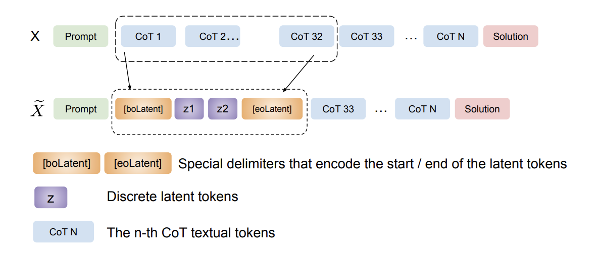
Figure 3.1Arxiv
During training, the VQ-VAE is shown the entire input sequence, but is only applied to the CoT tokens. The CoT sequences are gradually replaced with corresponding latent tokens. This, along with randomized replacement of text tokens with latent tokens, allows the model to adapt to using the latent tokens.
At test time, the model uses these “Z” latent tokens in its CoT. The VQ-VAE is only used for learning the tokens, and isn’t needed during inference.
As for results, the model showed an increase in reasoning ability, both in- and out-of-domain of the datasets they trained on. The increase in ability seems relatively small compared to other reasoning methods (~4% improvement vs. traditional CoT). The more interesting result is that the model was able to improve slightly in performance while using ~17% fewer tokens in its reasoning trace. So it seems like this method allows the model to develop a more efficient vocabulary for reasoning.
Overall, I’m not sure that the performance increase shown in Token Assorted is worth losing the visibility into the CoT.
Reasoning with Recurrence in Latent Space
Scaling up Test-Time Compute with Latent Reasoning: This paper introduces a novel way of reasoning in latent space, using a depth-recurrent transformer. Their model, “Huginn”, combines a traditional decoder-only transformer with a recurrent block, which can be iterated multiple times during decoding before emitting a token – allowing for the “reasoning” in latent space. Like s1’s budget policy, the number of thinking iterations can be selected at test time.
The high-level generation approach is, roughly, embed the input sequence into the latent space using a transformer layer (“Prelude”), then iterate this transformed input through a recurrent block for some number of iterations, then un-embed the final state into an output token (“Coda”).
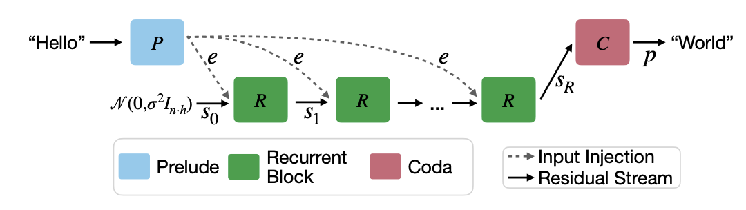
Figure 2Arxiv
There are a couple really cool results about this approach:
- The recurrent loops can be seen as a convergence process, where the model able to spend more “effort” generating a token. More iterations results in greater certainty in the output.
- The convergence framing allows for adaptive compute at inference time. By specifying a threshold difference between successive states in the recurrent portion, the model can keep iterating until it has converged on a token – allowing for more iterations on “difficult” tokens and fewer on “easier” tokens that converge more quickly.
As a hand-wavey intuition for this, assume you have some “distance” measure D
that allows you to determine the difference between two of the hidden states
used in the recurrence block. You can measure how much the model has updated
it’s “belief” for each recurrent iteration by calculating D(r_i, r_{i+1}). If
the model is reaching convergence, the value of D(r_i, r_{i+1}) will
monotonically decrease as i, the number of iterations, increases. You can set
some threshold T after which you stop iterating. Thus, if the model displays
uncertainty and takes many iterations to reach T, it has time to do so; but if
the model converges quickly to T, you don’t need to keep iterating once it’s
already converged.
There are two figures from the paper that illustrate this well:
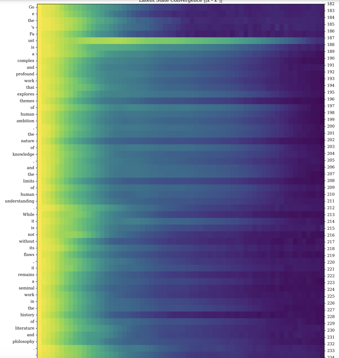
Figure 19Arxiv
In Figure 19, we see the model processing a query, with colors representing how much the model updated its hidden state with each recurrent iteration. The darker colors roughly indicate high convergence, and the lighter colors indicate low convergence. For most tokens in the sequence, the model converges quickly. The tokens between sentences, and in “Faust” here seem to indicate lower confidence, as even after several iterations the model doesn’t settle into a firm prediction.
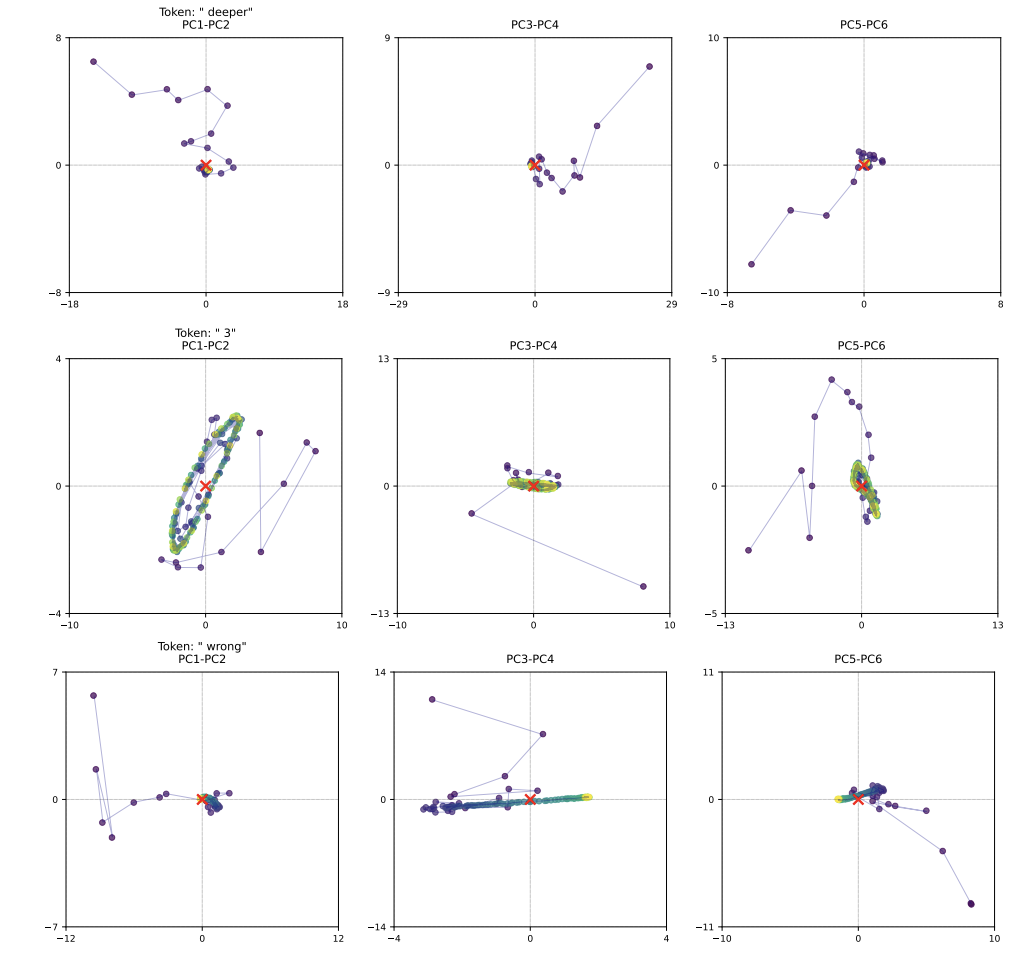
Figure 12Arxiv
In figure 12, we see a lower dimensional projection (via PCA) of the trajectory
of the latent space state for particular tokens. This is a way to visualize how
the hidden state evolves as it goes through more iterations. There are a bunch
of interesting behaviors here. In the first row, we see a straightforward
convergence to the center. For the second row, the token is the number 3, and
the model exhibits an “orbiting” pattern. And for the third row, the token
oscillates/slides in the second component. The paper authors infer that this
learned orbiting and sliding behavior allows handling of more advanced concepts.
(All of this was learned emergently and wasn’t part of the training objective!)
Another interesting component of this paper is that the do not require specialized datasets including CoT for their training. The training procedure is relatively complicated, so my summary will not do it justice. However, at a high level they run the recurrent block for a random number of iterations. So the model isn’t “locked” into a particular number of iterations – it is pushed to learn to use an arbitrary number of iterations on a particular generation.
Zero-Shot Continuous CoT:
By reusing the hidden state from the recurrence block between token decoding
steps, the model can use this hidden state as a reasoning “scratch pad”. For
example, when working on a task that requires reasoning, reusing this hidden
state seems to allow the model to reuse some of the partial work its done on
token i, such that during token i_1, it can recycle some of that work and
needs fewer iterations to converge.
Zero-Shot Self-Speculative Decoding:
Speculative decoding is a performance optimization which uses a cheaper “draft”
model to reduce the cost of decoding a more expensive model. This recurrent
model gets you something similar to speculative decoding “for free” without a
draft model. To do this, you can decode with a small amount of iterations N
and treat that as the draft model, and decode with a larger number of iterations
M as the ground-truth model. (So, M > N.) This has two efficiencies: First,
since the draft and ground-truth model use the same weights, you don’t have to
have two models loaded during inference. Second, the hidden states calculated in
the draft model (N iterations) can be reused by the ground-truth model when
decoding from [N+1 -> M] iterations.
Zero-Shot Adaptive Compute at Test-Time: As discussed earlier, you can use a
convergence threshold T when calculating the difference between recurrent
states, and stop after the threshold is reached. This allows per-token adaptive
compute, allowing the model to spend more compute on harder tokens.
The Bitter Lesson
With the release of o1/r1/o3, I’ve seen the sentiment of “Hey, this is further proof of the bitter lesson. Scaling English CoT is all you need to reach AGI”. Along with variants of: Mamba was a dead end, MCTS was a dead end, COCONUT is a dead end.
Mamba for sure hasn’t started “working” yet at the frontier, and I don’t see that changing soon. I don’t think MCTS should be ruled out yet, though it also hasn’t had a breakout moment. It’s still quite early for latent reasoning. The model development pipeline is long, and I’m confident that frontier labs are trying to make latent reasoning work — for the efficiency gains, if nothing else. In a world where inference costs will increasingly be a bottleneck, shaving off that much compute while maintaining or even slightly improving performance is quite appealing.
The initial takeaway from this wave of reasoning research is that we’re still in the early stages of understanding how to make models think effectively. While English CoT has set a high bar, early results in latent reasoning and adaptive compute suggest there’s still plenty of low-hanging fruit in making models reason more efficiently. The bitter lesson can point us where we’ll end up (“simple” architectures in hindsight, scaled massively), but there’s still much to learn about the best way to get there.
Cover image by Recraft v3.
-
It seems like the cutoff for models being able to learn reasoning ability is roughly in the 1.5B - 3B parameter range. But also the Qwen models seem much more capable of being transformed into reasoners than Llama, so there’s probably something other than raw scale going on here. ↩︎