
Recently, I’ve been reading through the excellent Database Internals (Alex Petrov, 2019). The first half of the book is dedicated to the implementation of database storage engines – the subsystem(s) of a DBMS that handles long-term persistence of data. A surprising amount of this section discusses the implementation and optimization of various B-Tree data structures.
In my college Data Structures and Algorithms course, we covered B-Trees, but I didn’t grok why I’d choose to use one. As presented, B-Trees were essentially “better” Binary Search Trees, with some hand-waving done that they had improved performance when used in database applications. I remember needing to memorize a bunch of equations to determine the carrying capacity of a M-degree B-Tree, and a vague understanding of B-Tree lookup/insertion/deletion, but not much else. Which is a shame! They’re interesting structures.
I this was partially a failure of visualization, and partly a failure of providing motivating examples. On visualization: Most B-Tree visualizations I’ve seen portray them more-or-less as n-ary trees, usually of degree 3-5. This is not wrong, but it obscures why you would actually use a B-Tree (e.g. in part, collocation of perhaps hundreds of keys in a single node).
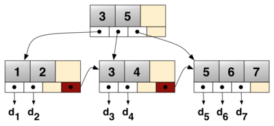
The Wikipedia article illustration of a B+ TreeSource: Wikipedia
The other failure, of motivating examples, could be solved by providing the following prompt: What do you do when a set of key/value pairs no longer fits in memory, and you want to design a disk-friendly structure to store them all?
[Caveat emptor] This post isn’t meant to be a comprehensive guide to B-Trees (I’d recommend Database Internals for something approaching that). Rather, here’s how I’d now explain the reasoning for why a data structure like a B-Tree is useful:
Disk-Induced Constraints
Consider we’re trying to store a large number of key-values pair on disk. We want an easy way to read them back, and we also want to be able to easily query for a specific key or range of keys. Once we introduce disk IO, we hit some constraints that aren’t typical of in-memory structures:
- Constraint: The entire dataset will not fit in memory.
- The effect: Data needs to be laid out such that traversing the structure is possible by loading only a subset of the structure into memory.
- Constraint: The smallest unit of storage that can be read/written
to/from a drive is large, compared to in-memory access (usually an entire
page vs. a single byte).
- The effect: Try to co-locate data likely to be accessed together as much as possible.
- Constraint: Disk I/O is significantly slower than in-memory lookups.
- The effect: Reduce the # of disk accesses as much as possible.
So, how do we start? Petrov begins with an illustrative example. Consider the naive approach where we store key/values in a Binary Search Tree (BST), and store that BST on disk:
If we wanted to maintain a BST on disk, we’d face several problems. One problem is locality: since elements are added in random order, there’s no guarantee that a newly created node is written close to its parent, which means that node child pointers may span across several disk pages.
Since binary trees have a fanout of just two, height is a binary logarithm of the number of the elements in the tree, and we have to perform O(log2 N) seeks to locate the searched element and, subsequently, perform the same number of disk transfers.
A naive on-disk BST implementation would require as many disk seeks as comparisons, since there’s no built-in concept of locality.
(p28-29, emphasis mine)
BSTs as on-disk structures fall flat on their face, because the number of key comparisons is roughly equal to the number of disk seeks.
Notice that there are two quantities which are important here: The number of key comparisons, and the number of disk seeks. The number of key comparisons needed to locate an entry scales with the size of our dataset, so there isn’t much we can do to influence that. However, we can influence the number of key comparisons enabled by each disk seek. How? By collocating keys together in the on-disk layout. What if, say, we stored a bunch of keys adjacent to one another on disk so that with one seek, we could perform a large number of key comparisons? Yup – that’s what we get with B-Trees. In other words, B-Trees have high fanout.
And this is why portraying B-Trees as 3-ary to 5-ary trees is misleading: we can actually store hundreds of keys per node, which only increases the comparisons-per-seek fanout benefit.
Slotted Pages
So far, so good. However, when reading deeper about B-Trees, the actual details about how keys are laid out on disk to maximize locality and key compaction made me appreciate this approach even more. Taking a step back, let’s recall from “CS common knowledge” some basics about persistent storage:
Hard Disk Drives (HDDs) contain spinning disks that are read from and written to by a static head. This makes random access slower than sequential access, since each time you want to view a different part of the drive, you need to wait until the disk rotates so that the portion you want to access is below the head.
Solid State Drives (SSDs) are built from a bunch of memory cells, composed into a hierarchy of pages, blocks, and panes. They have no moving parts, but each cell has a limited number of reads/write it can perform before becoming permanently inaccessible. So, there is device- and OS-level software to distribute operations across the drive, to extend the functioning life of the drive. Furthermore, SSDs aren’t just like “huge banks of slower RAM”, like my mental model had been previously. Rather:
The smallest unit that can be written (programmed) or read is a page. However, we can only make changes to the empty memory cells (i.e., to ones that have been erased before the write). The smallest erase entity is not a page, but a block that holds multiple pages, which is why it is often called an erase block. Pages in an empty block have to be written sequentially. (pg30)
All of this to say, both HDDs and SSDs have hardware constraints on the smallest unit they can read/write. The OS abstracts this as a “block device interface”. Why do we need to care about this? Any on-disk structures we create should be aware of the number of blocks (also called pages) that they change. Changing 1000 bytes in 1000 different blocks is going to be much slower than changing 1000 bytes in the same block. The same is true for read operations. Thus, we want the logical layout of our data structure to fit nicely within the block device abstraction.
B-Trees naturally lend themselves to be laid out in pages: each logical tree node gets a disk page. We can tune the parameters of the tree (primarily, the number of keys per node) so as to fix a node comfortably within a disk page.
However, B-Trees are dynamic. Tree nodes can change due to any insertion or deletion, and keys must stay in sorted order within nodes. How can we layout data in a sorted order without needing to move a bunch of data around during each mutation operation? The answer: Slotted pages.
Slotted pages are composed of three components: a header (containing metadata about the page), cells (variable-sized “slots” for data to be stored in), and offset pointers (an array of pointers to those cells).
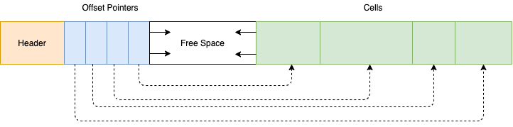
Slotted Page Layout
The benefit of this layout is that you can store variable sized data, since the cells can be of variable size, and you don’t need to move that data to logically reorder it. Reordering the positions of the pointers in the pointer array is sufficient. This is inexpensive since the pointers are small, and in a well-known position at the beginning of the page. In other words, as long as the offset pointers are ordered in key-sorted order, it doesn’t matter where in the actual page the keys are stored.
This means that you can also free and reuse cells as data is deleted/inserted. SQLite, for example, manages this with a freelist.1
B-Tree Lookup
There are a couple more optimizations I’d like to discuss, but before doing so it will be helpful to discuss how B-Trees perform lookups. The B-Tree lookup algorithm is pretty simple. It’s usually described as something like:
- Start at the root node.
- Look at the separator keys in the current node, to find the child node which would logically contain the search key you’re looking for.
- Recursively traverse the tree using the logic from step 2.
- If you hit a leaf node containing the key you’re searching for, you’re done. If you discover that a leaf node does not exist for the search key (e.g. there is no leaf for the range you’re seeking), or the leaf node does not contain the desired key, report that the key does not exist, and you’re done.
Step 2, however, glosses over several interesting details – which become more relevant with higher degree trees storing larger amounts of data. First: In most implementations when traversing the tree, you perform binary search on the keys within a node . This is why it’s so important that keys are store in sorted order within nodes. Second: Except for the leaf nodes, which actually store data2, the full value of the separator key isn’t important – it’s just acting as a partition between nodes. As long as the separator key accurately represents a partition between the key range each child node is responsible for, it can be any value which holds that partition property. Using one of the actual database keys as the partition key is just a convenient method of picking a partition key.
Separator Key Truncation
Taking advantage of the above insight, we can decide to use “better” partition keys to improve B-Tree storage efficiency:
We can save space in pages by not storing the entire key, but abbreviating it. Especially in pages on the interior of the tree, keys only need to provide enough information to act as boundaries between key ranges. Packing more keys into a page allows the tree to have a higher branching factor, and thus fewer levels. (Designing Data-Intensive Applications, Martin Kleppmann)
To illustrate this, suppose you’re trying to store the following keys:
0xAAAAAA
0xBBBBBB
0xCCCCCC
0xDDDDDD
0xEEEEEE
0xFFFFFF
… and our insertion algorithm has decided to store these in 2 tree nodes:
# Node 1
0xAAAAAA
0xBBBBBB
0xCCCCCC

# Node 2
0xDDDDDD
0xEEEEEE
0xFFFFFF
What should the parent of Node 1 and Node 2 use as the separator key between
them? The naive implementation would use 0xDDDDDD. Everything less than
0xDDDDDD is in Node 1, everything greater than or equal to 0xDDDDDD is in
Node 2. However, notice that there is a large gap between 0xCCCCCC and
0xDDDDDD. We can use a much less granular separator, and still maintain the
correct partition. For example, if we store the prefix “key” 0xD* as the
separator, this tells us just as much information, with fewer bytes needed to
store.
Recall that key length can be (effectively) unbounded, so this technique can save significant space in pathological cases. This is again a failure of visualization: most diagrams (for simplicity) show small keys – choosing single digits or characters. However, in a real database system, keys can be nontrivially large – SQLite has a default maximum key size of 1MB.3
Update: An excellent comment by spacejam on Lobste.rs points out that key prefix truncation is also a common practice, and can save more space in nodes that suffix truncation:
[P]refix compression [is] even more important than suffix truncation, because over 99% of all nodes in a db are leaves (assuming > 100 index fan-out, which is pretty common when employing prefix encoding + suffix truncation). Prefix compression saves a lot more space. Suffix truncation is still really important for index node density, and thus cache performance and pretty much everything else though. (Source)
Overflow Pages
With Separator Key truncation, we are able to pack more keys into internal (non-leaf) nodes by truncating keys. Sometimes, we may run into the opposite problem in leaf nodes: Our (physical) page is too small to fit the number of keys we are supposed to have in a (logical) node.
In this case, some B-Tree implementations turn to Overflow Pages. The storage engine allocates a new page for overflow data, and updates the first page’s header to indicate the overflow. My initial intuition would be that you’d just allocate extra cells in the overflowed page, and treat the whole thing as just “more cell space”. However, you can be a bit more clever by using the same insight from separator key truncation: most database operations are on key ranges, so having fast access to a key prefix can be more important than having access to the entire key.
So, it can be more efficient to actually split the key – storing the prefix in the original page, and overflowing the rest to the overflow page:
# Very long key:
AAABBBCCCDDDEEEFFFGGGHHH

| Stored in primary page | Stored in overflow page |
----------------------------------------------------
| AAABBBCC               | CDDDEEEFFFGGGHHH        |
This way, if we are checking for key presence or performing a range query, there’s a higher likelihood that we won’t need to consult the overflow page – since in many cases the key prefix is enough to answer a query.
Sibling Pointers
The last optimization I thought was particularly interesting was an extra bit of bookkeeping:
Some implementations store forward and backward links, pointing to the left and right sibling pages. These links help to locate neighboring nodes without having to ascend back to the parent. (Database Internals, pg 62)
These sibling pointers make range queries more performant:
During the range scan, iteration starts from the closest found key-value pair and continues by following sibling pointers until the end of the range is reached or the range predicate is exhausted. (pg38)
First: At a per-level basis, sibling nodes always have non-overlapping strictly increasing key ranges. This means traversing to a node’s right sibling is guaranteed to (at that level) contain the logically “next” chunk of the key space. Second: In deeper trees, having sibling pointers can mean preventing potentially many “reverse traversal” back up parent nodes.
To prove this to myself, consider the following diagram (with a binary tree, for simplicity). The first row in each node represents the key stored in the node, and the second represents the valid keys that can exist in that node:
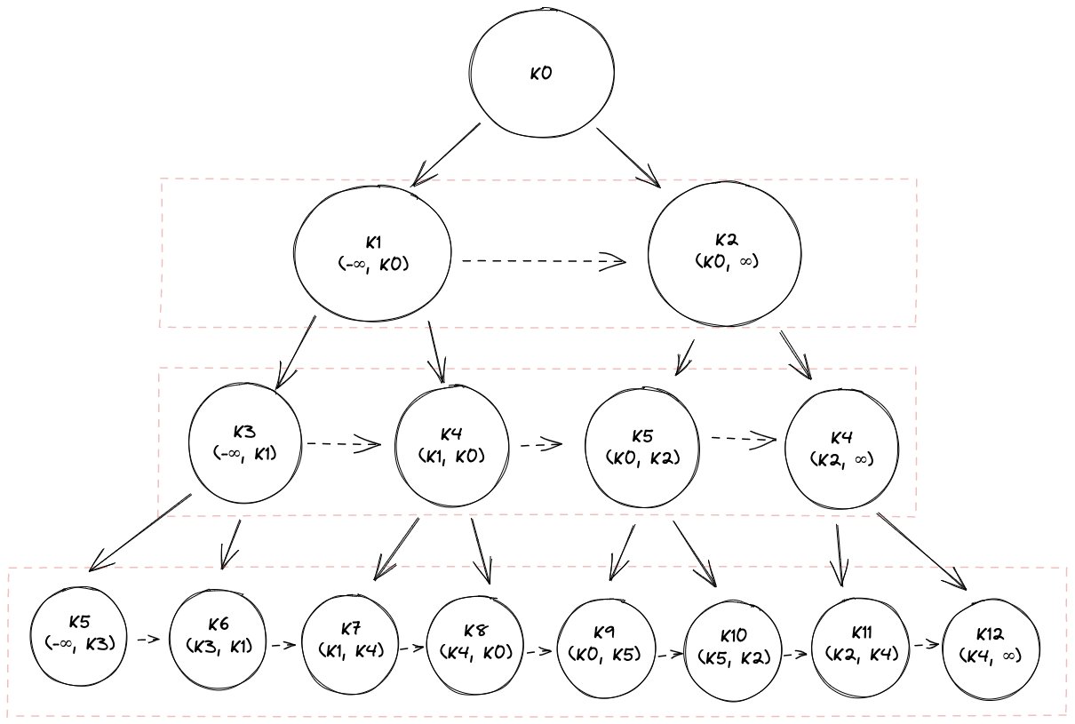
Visual proof for key range property of per-level siblings
Moving from K8 to K9 is one sibling pointer away, as opposed to six hops traversing up and back down the tree. So, when querying for a range of values, the additional sibling pointer bookkeeping can prevent a lot of unnecessary backtracking.
B-Tree Variants
Finally: Aside from B⁺-Trees, which is primarily what I’ve been discussing, there are variants of and optimizations to B-Trees that can provide optimizations in certain circumstances: “Lazy B-Trees” like WiredTiger and Lazy-Adaptive Tree can improve performance by buffering writes. FD-Trees structure B-Tree data in a fashion more friendly to SSDs’ physical characteristics. Bw-Trees (amusingly, “Buzzword trees”) provide further optimizations for high-concurrency and in-memory tree access.
Conclusion
If any of this stuck you as interesting, I’d again highly recommend reading through Database Internals. I think the biggest takeaway that I had is that there’s a significant difference between a data structure as an abstract mathematical concept (“a B⁺-Tree”) and concrete implementations (“SQLite’s database format”). Optimizations to concrete implementations won’t improve the BigO characteristics of a data structure, but will have significant “real world” implications on performance and usability of a database.
Also, all of this only begins a longer discussion about finer grained optimizations to specific storage systems. As I learned digging into Raft, the devil is in the details. “Some extra bookkeeping is required” is a ready invitation for maddening bugs and nontrivial complexity.
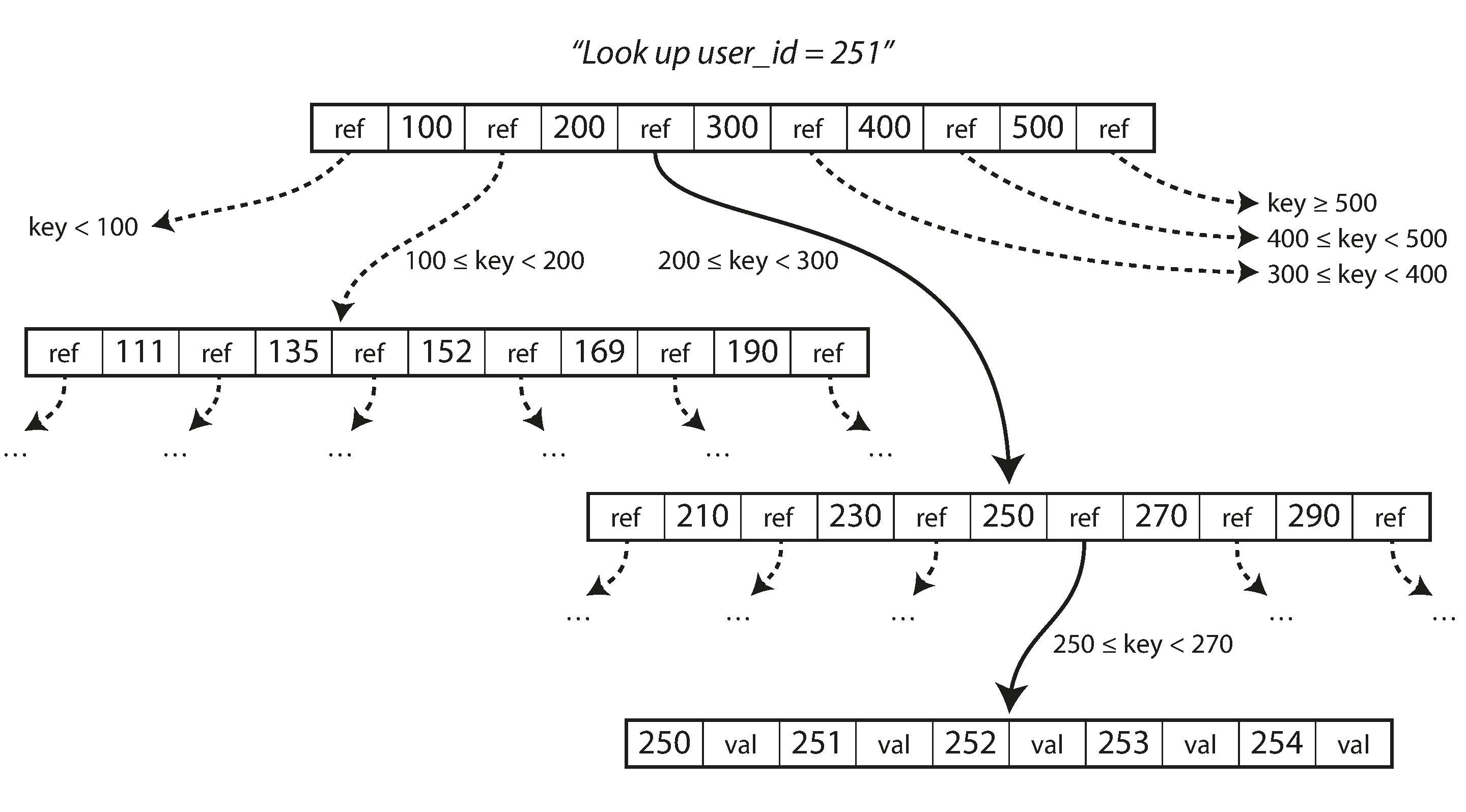
As a final note: Since I’ve been complaining about tree visualizations, I did find a B-Tree diagram that I think gives a better intuition as to in-practice tree structure. This is from Martin Kleppman’s Designing Data Intensive Applications:
Cover: Unsplash